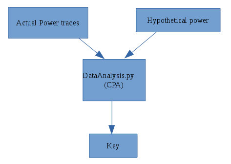
Running Correlation Power Analysis¶

One of the most used variants of Deferential Power Analysis (DPA) is Correlation Power Analysis (CPA). In this document, we show the theory behind CPA before showing concrete examples. This discussion follows the notation and concepts discussed in the book “Power Analysis Attacks - Revealing the secrets of Smart Cards” by Mangard, Oswald and Popp.

How CPA Works?¶

Correlation Power Analysis uses an intermediate value that is a function of part of the key and known data. The power consumption of the devices when the intermediate value is processed is estimated for each key guess. A statistical method is then used to find out which key was most likely used by correlating the hypothetical power and the real power consumption. below we discuss this process in detail.

CPA Flow

Step 1: Choose the intermediate value¶

We choose an intermediate variable that is processed in the algorithm. The intermediate value is calculated as f(d, k) Where d is a known non-constant value that can be derived from known data (e.g. plain text) and k is small part of the key.

Step 2: Power measurement¶

Measure the power consumption of the crypto device while it encrypts/decrypts D data blocks. We need to know the value d the corresponds to each data block. These values can be written as a vector d = [d₁, d₂, …, d_D]. The power consumption signal for a single encryption/decryption operation is called a trace. A trace is vector that records instantaneous power consumption for the time of interest (the time when the intermediate value is being processed). The trace generated while encrypting/decrypting data block i consists of T samples and can be viewed as a vector t_i = [t_i,1, t_i,2,… , t_i,T]. The traces are stacked in a matrix T with dimensions D x T where each row i is a trace generated while encrypting/decrypting block i.

Step 3: Calculate hypothetical intermediate¶

Next, we need to guess the key part that goes into the calculation of the intermediate value. We list all possible sub keys as a vector k = [k₁, k ₂ ,…., k_K]. Then, we calculate the intermediate value f(d, k) for all values in the vectors d and k. The result is stored in a D x K matrix V. Where

V_i,j = f(d_i, k_j)

and i = 1, 2, …D and j = 1, 2 …K

Note that each column in V is the intermediate value calculated for all data values d for one key guess.

Step 4: Calculate Hypothetical Power¶

Now we have calculated the intermediate values matrix V, we estimate the power consumption when each value in V is processed in the device. Two power models are widely used:

The Hamming Weight model (HW). this model counts the ones in the value e.g HW(1100 0000) = 2
The Hamming distance model (HD). This model counts the the number of bits that flips when a the value of a variable (e.g. register) changes. That is

HD(x, y) = HW(x xor y)

e.g HD(0000 0011, 0000 0101) = HW(0000 0011 xor 0000 0101) = HW(0000 0110) = 2

The result is a D x K matrix called H. These are the same dimensions as the matrix V.

Step 5: Correlate the hypothetical power and the real power traces¶

We correlate H and T to find the key. The question is: which column in V was most likely processed in the device? We use a correlation algorithm that takes two vectors as input and returns a real number that measures how ‘similar’ the vectors are. Each column i in H is compared with column j in the trace matrix T. The result is stored in the correlation matrix R which is a K x T matrix. Note that column i in matrix H is the hypothetical power if k_i is used in the device and column j in T is the real power measurement at sample j for all data blocks.

The element R_i,j measures how similar the column i in H to column j in T. The index of the highest element in the matrix R ck, ct are the in index of the key and the sample in time of the supposedly correct key since it indicates that the corresponding columns in H and T are similar so it is likely that the guessed key was indeed used in the device.